Aggregate demand and aggregate supply

Aggregate demand (AD)

The total planned expenditures (spending) by households, firms, government and foreign sector in a period of time at given price levels.

Why AD curve is downward sloping

• The wealth effects: Price level ↑ → real income ↓ → C & I ↓ → Real output ↓
• Interest rate effect: Price level ↓ → Interest rate ↓ → C & I ↑ → Real output ↑
• International substitution effect: Domestic price level ↓ → Relative PM ↑ & PX ↓ → Real output ↑

Shift of AD curve affected by

Changes in consumer spending

1. Consumer confidence:
2. Interest rate
3. Personal income tax
4. Level of household indebtedness

Changes in investment spending

1. Business confidence
2. Interest rate
3. Business taxes
4. Level of corporate indebtedness
5. Improvement in technology

Changes in government spending

1. Political priorities
2. Economic priorities (deliberate efforts to influence aggregate demand)

Change in foreigner’s spending

1. Changes in national income abroad
2. Changes in exchange rates
3. Changes in level of trade protection

Aggregate supply (AS)

The total quantity of goods and services produced in an economy (real GDP) over a particular time period at different price levels.

Why SRAS is upward sloping

Profitability (Price, output,cost remain constant. profit, incentives of production, real out put)

Shift of SRAS curve affected by

• Change in cost of production
• Change in business taxes & subsidies
• Supply shock – natural disaster

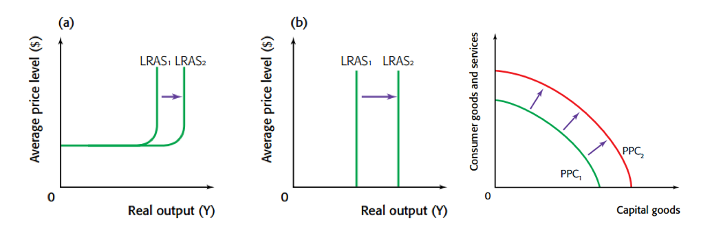
Long-run aggregate supply (LRAS)

The aggregate quantity of goods & services supplied when the economy is operating at full employment.

Shift of LRAS curve affected by

Quality and quantity of factors of production

Full employment level of output (Yf)

The output level that is produced by an economy when labour market is in equilibrium and thus there is only natural unemployment. It also represents the potential output that could be produced if the economy were operating at full capacity.

Full employment output Yf (LRAS) = potential output (PPC)

Short run

The period of time when prices of resources are roughly constant or inflexible (they do not change much in response to supply and demand), such as wage

Long run

The period of time when the prices of all resources, including the price of labour (wages), are flexible and change along with changes in the price level.

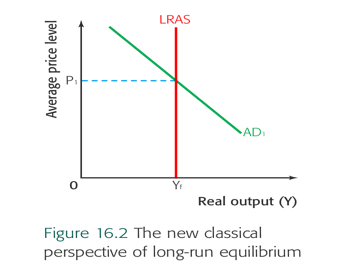
New classical (neo-classical) economics

Include different branches such as monetarist, supply-side economics. These economists believe in the efficiency of market forces and minimal government intervention in the resources allocation in the economy. Thus, it is known as free market economists and the followers of Adam Smith.

New classical LRAS curve is vertical (perfectly inelastic) at the level of potential output (full employment output Yf).

Reason

• Yf depends on the quantity & quality of the FoP.
• AS in LR is independent of the PL. (In LR, no unempt of resources because markets will clear. Thus, whatever PL, firms will supply maximum capacity of the economy.)

LR equilibrium in the new classical/ monetarist model

• AD = LRAS at full employment
• Changes in AD will only affect price level, NOT output level

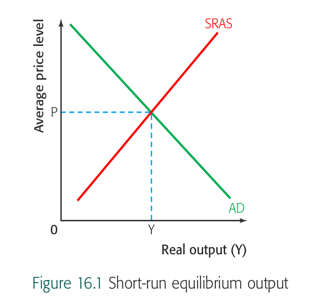
Short-run equilibrium

The economy is in SR equilibrium where AD=SRAS, producing an output level of Y at the price level of P.

• Output = total D: no reason for producers to change output/P
• AD=AS: no upward (inflationary) /downward (deflationary) pressure on PL
• As long as nothing changes to influence AD/AS, e. rests at E.
• Any changes in AD/SRAS (shifts) will move e. to a new E.
• This may NOT coincide with the FE level of output

Keynesian economics

It was established by the famous economist John Maynard Keynes and developed by his followers. These economists believe in government intervention and its core is demand management policies.

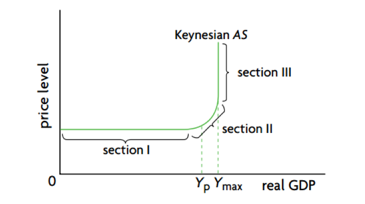
Keynesian model does not distinguish b/t SR & LR.

"Wage/price" downward inflexibility

• Wages are “sticky downwards” because firms find it difficult to cut wages (discontent & reduced motivation; L regulations, contracts; trade union power)
• Prices are “sticky downwards” because firms avoid lowering their prices (reduce profits if wages do not go down. Oligopolistic firms fear price war.

Keynesian AS curve has three sections

1. Horizontal (perfectly elastic): with plenty of spare / excess capacity, economics operates at low output during depression. Firms can raise output without pushing up ACs.
2. Upward-sloping: economy approaches its potential output. As spare capacity is “used up”, FoP become increasingly scarce. Firms have to bid for factors to increase output. As output increases, factor Ps (CoP) go up & PL will also rise.
3. Vertical (perfectly inelastic): economy reaches its full capacity (physical limit Yf). Impossible to raise output as all FoP are fully employed.